I’ve recently returned to my hledger scripts from the memo “Visualise your finances with hledger, InfluxDB, and Grafana”, and in particular adding support for multiple currencies.
This got me thinking about market values. If I want to see the current market value of all my assets, I need to convert them all to the same currency, using a recent exchange rate. So I now have a script to fetch, once a day, exchange rates between £ and everything else:
P 2018-05-30 BTC £5501.58
P 2018-05-30 ETH £413.01
P 2018-05-30 LTC £87.85
P 2018-05-30 EUR £0.8775
P 2018-05-30 JPY £0.0069
P 2018-05-30 USD £0.7531
P 2018-05-30 VANEA £210.24
My script exports market values to influxdb, so I can see how the market value of my assets (in £) has changed over time. Great!
But what if I want to see the market value in a currency other than £? Like USD, for instance? The problem is that I have all these exchange rates:
digraph {
  BTC   -> £ [label="* 5501.58"]
  ETH   -> £ [label="* 413.01"]
  LTC   -> £ [label="* 87.85"]
  EUR   -> £ [label="* 0.8775"]
  JPY   -> £ [label="* 0.0069"]
  USD   -> £ [label="* 0.7531"]
  VANEA -> £ [label="* 210.24"]
}
But I don’t have, say, the exchange rate from EUR to USD.
Well it turns out that the reflexive-symmetric-transitive closure of that graph is just the thing I want! It looks pretty nasty with 7 currencies, so here it is with just 3:
digraph {
  £ -> £   [label="* 1"]
  £ -> BTC [label="* ?"]
  £ -> ETH [label="* ?"]

  BTC -> £   [label="* 5501.58"]
  BTC -> BTC [label="* 1"]
  BTC -> ETH [label="* ?"]

  ETH -> £   [label="* 0.8775"]
  ETH -> BTC [label="* ?"]
  ETH -> ETH [label="* 1"]
}
Let’s see how to calculate those ?s.
Representing graphs
I could pull in a functional graph library, but the graphs I’m dealing with are so small that I may as well just implement the few operations I need myself.
A graph is essentially a function node -> node -> Maybe label:
import Data.Map (Map)
import qualified Data.Map as M

type Graph node label = Map node (Map node label)
We need an empty graph and, given a graph, we need to be able to add nodes and edges. As our nodes are the keys in the map, they need to be orderable.
-- | A graph with no nodes or edges.
empty :: Ord n => Graph n l
empty = M.empty

-- | Add a node to a graph.
addNode :: Ord n => n -> Graph n l -> Graph n l
addNode n = M.insertWith (\_ old -> old) n M.empty
We don’t allow duplicate edges, as that means we have two exchange rates between the same pair of currencies, which doesn’t make much sense. So adding edges is a little more involved, as the edge might already exist:
-- | Add an edge to a graph, combining edges if they exist.
--
-- If the source node doesn't exist, does not change the graph.
addEdge :: Ord n
  => (l -> l -> l)  -- ^ Function to combine edge labels.
  -> n  -- ^ Source node.
  -> n  -- ^ Target node.
  -> l  -- ^ New label.
  -> Graph n l -> Graph n l
addEdge combine from to label graph = case M.lookup from graph of
  Just edges ->
    let edges' = M.insertWith combine to label edges
    in M.insert from edges' graph
  Nothing -> graph
Computing the closure
Ok, so we can represent our currency graph. Now we need to compute the reflexive-symmetric-transitive closure.
Reflexivity lets us go from a currency to itself:
-- | Take the reflexive closure by adding edges with the given label
-- where missing.
reflexiveClosure :: Ord n => l -> Graph n l -> Graph n l
reflexiveClosure label graph = foldr (.) id
  [ addEdge (\_ old -> old) nA nA label
  | nA <- M.keys graph
  ] graph
If we know a exchange rate from A to B, symmetry gives us an exchange rate from B to A:
-- | Take the symmetric closure by adding new edges, transforming
-- existing labels.
symmetricClosure :: Ord n => (l -> l) -> Graph n l -> Graph n l
symmetricClosure mk graph = foldr (.) id
  [ addEdge (\_ old -> old) nB nA (mk lAB)
  | (nA, edges) <- M.assocs graph
  , (nB, lAB) <- M.assocs edges
  ] graph
If we know an exchange rate from A to B, and from B to C, transitivity gives us an exchange rate from A to C:
-- | Take the transitive closure by adding new edges, combining
-- existing labels.
transitiveClosure :: (Ord n, Eq l) => (l -> l -> l) -> Graph n l -> Graph n l
transitiveClosure combine = fixEq step where
  fixEq f = find . iterate f where
    find (a1:a2:as)
      | a1 == a2 = a1
      | otherwise = find (a2:as)

  step graph = foldr (.) id
    [ addEdge (\_ old -> old) nA nC (combine lAB lBC)
    | (nA, edges) <- M.assocs graph
    , (nB, lAB) <- M.assocs edges
    , (nC, lBC) <- M.assocs (M.findWithDefault M.empty nB graph)
    ] graph
Putting it all together
Exchange rates have three properties which we can make use of:
Any currency has an exchange rate with itself of 1.
If we have an exchange rate of
xfrom A to B, then the rate from B to A is1/x.If we have an exchange rate of
xfrom A to B, and an exchange rate ofyfrom B to C, then the rate from A to C isx*y.
So, given our graph of exchange rates, we can fill in the blanks like so:
-- | Fill in the blanks in an exchange rate graph.
completeRates :: (Ord n, Eq l, Fractional l) => Graph n l -> Graph n l
completeRates =
  transitiveClosure (*) .
  symmetricClosure (1/) .
  reflexiveClosure 1
There’s also a fourth property we can assume in reality:
- Any two paths between the same two currencies work out to the same exchange rate.
Otherwise we could make a profit by going around in a circle, and I’m sure someone would have noticed that already and made a lot of money. In our implementation however, we can’t assume that. Exchange rates available online have limited precision, and rounding errors will introduce more problems. But in general things will be close, so it doesn’t matter too much from the perspective of getting a rough idea of our personal finances.
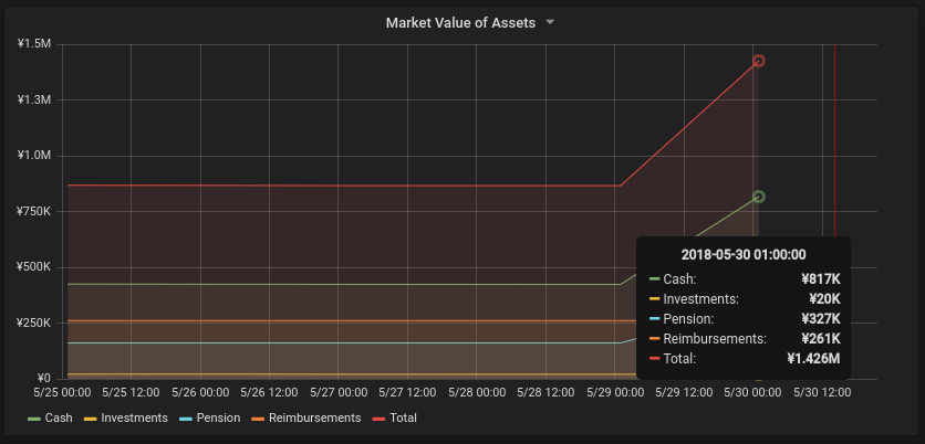
So now I can look at my total assets in yen and feel like a millionaire: